Access/Egress and PT Times Relation (ICR >0.5)
Access and egress times are related to public transport time (Fig. 12) in two ways as shown earlier in Eqns. 15a and 15b. The negative sign in Eqn. 15b suggests that a station which is not necessarily the closest (or within limits) from the first origin of the intended trip may be accessed to perform the trip by public transport. That is, a station with a travel time of TA may be accessed, if within PAZ, against the station with a lower travel time of Ta, skipping some closer stations, resulting in a lower PT travel time of Tp against the higher PT travel time of TP. In the return trip the same will be egress times from first destination. It is also possible high access and egress times to be prevalent at terminal stations on the periphery for users originating from or destined to locations that are far away in the outward direction from the station.

Example: A study at a park and ride facility, of transit service, in a suburban area in Seattle (Washington, USA) observed about half of its demand is generated in an area of 4-km radius of the facility and a large part of the remainder is generated from a parabolic shaped area (with a chord length of 16 to 20 kms) extending up to 16 kms upstream of the facility [34]. And, also the access distances of 30 and 50 kms reported in Rio de Janeiro, Brazil (Metro) [30].
Inter Connectivity and Co-Modality
“Co-modality refers to the use of different modes on their own and in combination in order to obtain an optimal mobility outcome in terms of travel effort as well as transport sustainability and supply efficiency” [36].
The total transportation time between an origin and a destination; in addition to travel time by PT, access and egress modes; includes; ticketing, waiting, dwell (boarding/ alighting) and transfer times.
Including these terms, an updated equation (Eqn. 40); for Inter Connectivity Ratio – indicating the indicator’s limitations (as defined by Eqn. 14) to capture the many dimensions of co-modality – addressing, at least partially, the quality of interconnection for measuring the share of ‘interconnectivity time’; was suggested in [36].

Considering transfer time and other component terms, Eqns. 10, 15 and 17 will change to:


Comparison of Different ICRs and Desirable ICR
The updated ICR (Eqn. 40) considered time in system, ts, in the numerator and denominator, as the components of PT system represented by it are an interface between access/ egress modes and PT modes. However, if it is considered only in the denominator, as suggested in Eqn. 46, that is alternate definition of ICR, the interface characteristic of it will be absent although it fulfils the requirement of considering all components associated with PT system.

Interconnectivity values by the three formats of ICR will be different and their relationship is:

However, ICR(t) may be useful in quick estimate of inter connectivity in case of non-availability of time in system. And; ICRa(t), the alternate ICR, has no significant advantage over ICR(t), for both estimate the same access/egress distances.
Characteristics of Index of Co-Modality (ICM)
Two indices of co-modality in time and cost terms are:


ICM is lower with improvements in travel time by PT mode (

Thus, interpretation of ICM values pre and post changes in any of the components of PT system should consider whether the changes are; in, (a) any/some/all of access, egress and time in system components only or, (b) is related to PT mode only or, (c) in both (a) and (b). These multiple cases result in dual interpretation of ICM.
Lower ICM value is appropriate from the user’s perspective in cases; such as, extension of a corridor positively impacting (minimizing) access/egress distance(s)/time(s) in the areas thus connected, changes in ticketing from manual to electronic reducing ticketing time, frequency of service reducing waiting time and any other system improvement measures. That is, from user’s perspective lower the ICM the better the service.
However, improving the speed of the service resulting in reduction in PT travel time with no improvement in access related activities in the system and thereby resulting in higher ICM values is better from system’s perspective and is common to all users.
If the increase in PT speed also results in the decrease of waiting time due to increased frequency it will result in a lower ICM value.
Also, PT network expansion with additional interchange nodes reduces PT travel time, thereby, increasing the index value for some users and reducing the index value for some users due to improvements in access/egress times.
Access/Egress Distances and Travel Direction Deviation


Access/Egress/PT Travel Distances (TAELETP)
The maximum (tolerable) limiting access or egress distance of a particular mode is that estimated considering the AM of speeds of access and egress modes (Eqns. 24-26). The general form of time-based limiting distance (Eqns. 23a-c and 26a) of any access or egress mode (m) is:


The chord length (based on Eqns. 8 and 50c), between the two ends of the arc (Long Chord), of an hexadecant sector (22.5o) of base trip length radius is:

The ratios of estimated limits of access/egress distances (based on both time and cost) to the arc length of the hexadecant sector of base trip length radius are:

1. The time-based estimated limits of access/egress distances exceed the arc length of an hexadecant sector of base trip length radius, if;
access/egress mode speed > 1.57 x base mode speed
2. The cost-based estimated limits of access/egress distances exceed the arc length of an hexadecant sector of base trip length radius, if;
base mode rate > 1.57 x access/egress mode rate
Eqn. 50c and ratios of speeds and rates in Eqns. 51 suggest:
1. The corresponding estimated limits of access/egress distances (time or cost based) exceed the arc length (equal to 39 percent of the base trip length) of an hexadecant sector of base trip length radius, in cases where, the respective ratios of speeds and rates (cost per unit of distance) of base and access/egress modes exceed 1.57;
2. If the respective ratios of speeds and rates are between 1.00 and 1.57, the corresponding estimated limits of access/egress distances are between a quarter (25 percent) of the base trip length and the arc length (equal to 39 percent of the base trip length) of an hexadecant sector of base trip length radius; and
3. If the respective ratios of speeds and rates are short of 1.00, the corresponding estimated limits of access/ egress distances are short of a quarter (25 percent) of the base trip length.
The limiting access and egress distance estimates (geometrical, not path) based on travel time, at origin and destination ends, are less than the arc length of the hexadecant sector considering the base trip length as the radius. This is true for all motorized base modes and any mix of access and egress modes as evident from the values of the ratios of speeds which are all less than 1.57 for any pair of motorized base modes and any access or egress modes (Appendix-1b).
However, the same is not true in the case of the limiting distance estimates based on travel cost, for, the values of the ratios of rates are greater than 1.57 for some pairs, such as, base modes – Auto rickshaw and Car – and access/egress modes – Bus and Motor cycle. The ratio is also higher than 1.57 in the case of Motorcycle as base mode and Bus as access/egress mode (Appendix-1b).
Eqns. 19b and 25c based on travel time and; Eqns. 29b and 35c based on travel cost suggest that the respective limiting sums of access and egress distances would be estimated by Eqns. 23d and 32d.
These equations and Eqn. 50c suggest that the ratios of estimated limiting sums of access and egress distances, based on both time and cost, to the arc length of the hexadecant sector of base trip length radius are:

1. The corresponding estimated limits of sums of access and egress distances (time or cost based) exceed twice the arc length (39 percent of the base trip length, the maximum limiting distance of access and egress modes individually) of an hexadecant sector of base trip length radius; i.e. 78 percent of base trip length, in cases where, the respective ratios exceed 3.14 ;
2. If the respective ratios are between 2.00 and 3.14, the corresponding estimated limits of sums of access and egress distances are between 50 and 78 percent of the base trip length;
3. If the respective ratios are between 1.57 and 2.00, the corresponding estimated limits of sums of access and egress distances are between 39 and 50 percent of the base trip length;
4. If the respective ratios are between 1.00 and 1.57, the corresponding estimated limits of sums of access and egress distances are between 25 and 39 percent of the base trip length; and
5. If the respective ratios are less than 1.00, the corresponding estimated limits of sums of access and egress distances are less than 25 percent of the base trip length
And, the ratios (based on speeds adopted Appendix-1d) are less than 3.14; so, it would be appropriate to assume that the maximum sum of access and egress distances would be 78 percent of the base trip length.
Also, the ratios based on rates (Appendix-1d) for some access-egress mode mix are less than 3.14, indicating that the rate based limiting sum distance estimates for such pairs would also be less than 78 percent of the base trip length.
Eqns. 52a and 52b give the relationship between limiting access and egress distance estimates based on travel time and travel cost.

That is, deviation angles for different overall limiting distances of all access/egress modes for all motorized base modes are less than the angle (22.5o) of an hexadecant sector of base trip length radius. This is at least true with the example set of speeds and corresponding rates of different modes assumed in Appendix-1a and needs to be examined with prevailing speeds and corresponding rates in different geographies or urban areas.
Eqns. 16a-h suggest a range of PT trip distances:


Access/Egress/PT Travel Distances (TAEGETP)
Eqn. 18 indicates the maximum travel time by public transport, corresponding to access/egress travel time, and therefore, the limiting PT distance would be:


1. is less than 0.785, then the travel distance by PT mode would be less than the arc length of an hexadecant sector of base trip length radius (i.e., 39 percent of the base trip length);
2. is between 0.785 and 1.57, then the travel distance by PT mode would vary between the arc length of an hexadecant sector of base trip length radius (i.e., 39 percent of the base trip length) and its double;
3. is between 1.57 and 2.00, then the travel distance by PT mode would vary between the double of the arc length of an hexadecant sector of base trip length radius (i.e., 78 percent of the base trip length) and base trip length;
4. is greater than 2.00, then the travel distance by PT mode would be greater than the base trip length; and
5. is greater than 3.57, then the travel distance by PT mode would be greater than the sum of the base trip length and twice the arc length of an hexadecant sector of base trip length radius (i.e., >1.785 – 178 percent of the base trip length).
That is, travel distance by metro (PT mode) based on travel time would be 0.65 times of base distance to same as base distance, and; 1.66 to 2.55 times of the length of the arc of an hexadecant sector; based on the ratios (Appendix-1e) of speeds of the PT mode and motorized base modes varying between 1.30 (car) and 2.00 (auto rickshaw).
And, the travel distance by metro (PT mode) based on travel cost would be 0.20 to 1.80 times of base distance, and; 0.51 to 4.58 times of the length of the arc of an hexadecant sector; based on the ratios (Appendix-1e) of monetary rates of motorized base modes and PT mode varying between 0.40 (bus) and 3.60 (auto rickshaw).
Eqns. 16g-o suggest a range of access-egress trip distances:


Eqns. 54a and 57b estimate the limiting sum of access and egress distances which delineates the two groups, TAELETP and TAEGETP for any pair of access-egress mode mix. Similarly, Eqns. 54b and 57a estimate the limiting PT distance that delineates the two groups, TAELETP and TAEGETP for the same pair of access-egress mode mix. In fact, the latter is true for all pairs of access-egress mode mix with the same base mode (Appendix-1f). Limiting sum of access and egress distances is higher for an access-egress mode mix with higher estimating ratio of modes in the mix.
Estimates of limiting sums of access and egress distances of any particular access-egress mode mix corresponding to TAELETP group is the distance that can be travelled in the limiting time (half of base trip time) for this group. That is, the range of access and egress distances in this group is from nil (i.e., PT availability at both origin and destination nodes) to the estimated limit. And; the range of distance for the same access-egress mode mix in the TAEGETP group will be between this limiting distance of the TAELETP group to its double (limited to base trip distance resulting in time savings) that can be travelled in a time equal to base trip time. That is, in the extreme case, a trip between an origin and destination can be completed by modes other than PT. This is also true in the case of distance estimates based on travel cost and the corresponding discriminant groups (Appendix-2) delineating the distances that are within the group CAELECP (ca + ce <= cp) or within the other group CAEGECP (ca + ce >= cp).
The range of limiting access and egress distance estimates of the discriminant groups TAELETP and CAELECP (Appendix-1f) suggest that some of the estimates are greater than the base trip length and can be limited to this value. This is especially, true of modes with corresponding estimating ratios greater than 4.00. Such trip lengths that are estimated by lower estimating ratios belong to TAEGETP and CAEGECP discriminant groups.
In practice sum of access and egress mode distances can at the most be equal to base trip length. In fact, much less, as these estimates are tolerable distances (maximum of the concerned range) and users prefer desirable and acceptable access/egress distances (minimum and mean of the concerned range) defined earlier. Additionally, considering Eqns. 42b and 45 these estimates will be further lower. And, thus; result in both time and cost benefits.
If access and egress nodes (PTNs) are within the limiting circles (PAZs), then access and egress distances will individually be less than or equal to 39 percent of the base trip length. That is, they are within the inner semi-circles of PAZ spread across, at the top end, of the hexadecant sectors around base travel direction. Or, within the outer semi-circles outside of the hexadecant sectors.
If either of access and egress nodes or both are outside the limiting circles (PAZs), then they must be within the central area, the space between the two inside semi-circles bounded by two common tangents of the two limiting circles (PAZs) joining them on the outside, which includes the hexadecant sectoral area (with deviation angles less than 22.5o) and an area outside of it. In these cases, sum of access and egress distances exceed 39 percent of base trip length and extend up to base trip length and over.

Minimum and maximum PT limiting distances when PTNs are on the extreme ends on the inside semi-circle and outside semi-circle respectively of the largest limiting circles on the line of base travel direction; i.e., the distances between “a1” and “e1” and; “a8” and “e8” are:

Perimeter of the Travel Envelope is:


The PT travel distance (1.78 times of base distance) between “a8” and “e8” (referred earlier) is a straight-line distance and is the inherent assumption, for PT and access/egress distances, in the model discussed thus far.
However, the stadia shape and the limits of access/egress distances suggest the possibility of considering a geometrical path other than the straight line for PT corridors (potential distances greater than 1.785 times the base distance within the limiting times) as PT corridors are both linear and circular.
That is, e.g. Purple Line (Fig. 15a) around the travel envelope and passing through “a8” and “e8”. The geometrical distance of purple line between these nodes (“a8” and “e8”) around the top edge of the Travel Envelope is greater than 2.234 times the base distance (which is half of the perimeter of the Travel Envelope).
Another example could be of an “n”-shaped PT corridor following an alignment along nodes “n1-a5-a3-e9-e3-n2” with a distance of about 1.785 times the base distance.
These may be considered as geometrical detours between any two such nodes; akin, to the detour of actual travel paths between any two nodes.
The latter example is a possibility with nil access/egress distances or a direct PT travel between nodes “n1” and ‘n2”. However, the first example of extreme length PT travel between the two nodes “n1” and ‘n2” would be a rare case and is a possibility in exceptional circumstances with exceptionally high access/egress distance (equal to the limiting distance at both the ends) appropriate for modes with a PT distance estimating rate ratio between 3.57 and 4.47 (Appendix-1e).
Another example of an extreme case with the same access/egress distance would be the one with a PT travel between nodes “a1 and e1” which is the least PT travel distance referred earlier.
The two examples of PT travel with both access and egress distances equal to the limiting distance facilitate a transfer across a traffic barrier (a congested bridge over a water body, access controlled at-grade railway crossing or any other) in any section (e.g. “a1 and e1”) along the desired travel path between nodes “n1” and ‘n2”. This is akin to a boat transfer across shores.
That is, the choice of PT mode, to fulfil the travel need between nodes “n1” and ‘n2” other than the direct (base) mode, would be based on travel time or travel cost or both depending on the alignment of the PT corridor(s), among several possibilities Fig-15a, serving in the Travel Envelope with access and egress nodes within the inner semicircles or in the outer semicircles. And; also, whether the access/egress nodes are within a particular mode’s overall limiting distances or outside.
PT Travel Distance Estimate
Travel distance by PT of a trip depends on the location of access (PTN-O) and egress (PTN-D) nodes within the travel envelope. That is, within respective PAZs or outside within travel envelope (central area – CATE – between the two PAZs at origin and destination ends).
PT travel distance for a trip can be estimated by the diagonal of a quadrilateral defined as:
The line representing base travel direction between an origin-O and a destination-D and the definition of deviation angles (Fig. 13) for PT travel results in a quadrilateral (origin-O, access-node-P, destination-D and egress-node-M, Fig. 15b)). The length (“p” to be determined) of PM which is one of the diagonals of the quadrilateral gives the PT travel distance with the other diagonal (of length “b”) being the base trip OD.
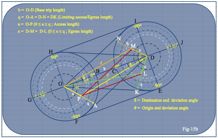
Using the formula for product of diagonals of a quadrilateral by Carl Anton Bretschneider [39], “p” can be estimated by Eqn. 60.

b = OD - Base trip length
q = OA = DN = DK = (π÷8)b
a = OP (0 <= a <= q, Access length)
e = DM = DL (0 <= e <= q, Egress length)
c = PD - Access node to destination length
d = OM - Egress node to origin length
𝛿 - Destination end deviation angle
𝜃 - Origin end deviation angle
𝛼 - PT node (SO) angle to base travel direction at FO end
𝛽 - PT node (FD) angle to base travel direction at LD end
This definition estimates PT distance for PTNs within PAZs.
If any of PTNs (PTN-O or PTN-D or both) are in CATE, the following changes, as appropriate, are necessary in constraints of the relevant parameters (that consider perpendicular distance to base travel direction) for estimating PT distance.
𝛼 - (-90 <= 𝛼 <= 90)
𝛽 - (-90 <= 𝛽 <= 90)
a - (a > q, 0 <= a x Sin(𝛼) <= q, Access length)
e - (e > q, 0 <= e x Sin(𝛽) <= q, Egress length)
Based on law of sines (Appendix-3) from ∆


That is, Eqn. 65 measures the straight-line distance between PTNs (SO and FD), if any, within PAZs of FO and LD.
Changing the location of access point “P” (Fig. 15b) results in change of shape from a quadrilateral to a triangle, and; also the line “PM” measuring the PT travel distance changes from a diagonal of a quadrilateral to a side of another quadrilateral or the side of a triangle depending on the location of the egress node at point “M” or “L” or any other point.
Case-1 – a = 0, e = 0, i.e. 𝛼 = 0, 𝛽 = 0
This results in access point “P” moving to origin “O” and egress point “M” moving to destination point “D”.
Therefore, Eqn. 65 reduces to:

Case-2 – 𝛼 = 0, 𝛽 = 0
This results in access point “P” moving to a point on the line segment OD at a distance “a” from origin “O” and egress point “M” moving to a point on the line segment OD at a distance “e” from destination point “D”.
Therefore, Eqn. 65 reduces to:

Case-3 – a = 0, i.e. 𝛼 = 0
This results in access point “P” moving to origin “O” and the line segment PM coinciding with the line segment OM making the PT travel distance measuring line segment a side of the
Therefore, Eqn. 65 reduces to:

Case-4 – 𝛼 = 0
This results in access point “P” moving to a point on the line segment OD at a distance “a” from origin “O” making the PT travel distance measuring line segment PM a side of the
Therefore, Eqn. 65 reduces to:

Case-5 – e = 0, i.e. 𝛽 = 0
This results in egress point “M” moving to destination “D” and the line segment PM coinciding with the line segment PD making the PT travel distance measuring line segment a side of the
Therefore, Eqn. 65 reduces to:

Case-6 – 𝛽 = 0
This results in egress point “M” moving to a point on the line segment OD at a distance “e” from destination “D” making the PT travel distance measuring line segment PM a side of the
Therefore, Eqn. 65 reduces to:

Case-7 – 𝛼 > 0, 𝛽 > 0
In this case, the line segment PM measuring the PT travel distance, through Eqn. 65, will be between a point in the 1st or 2nd quadrant of the limiting circle at origin end and that in the 1st or 2nd quadrant of the limiting circle at destination end cutting across the base trip travel direction.
Case-8 – 𝛼 < 0, 𝛽 < 0
In this case, the line segment PM measuring the PT travel distance, through Eqn. 65, will be between a point in the 3rd or 4th quadrant of the limiting circle at origin end and that in the 3rd or 4th quadrant of the limiting circle at destination end cutting across the base trip travel direction.
Case-9 – 𝛼 < 0, 𝛽 > 0 OR 𝛼 > 0, 𝛽 < 0
In this case, the line segment PM measuring the PT travel distance, through Eqn. 65, will align with line segment PL or the corresponding line segment on the opposite side of the base trip travel direction depending on which angle is positive or negative making it a side of a quadrilateral and the opposite side to base trip travel direction. The term involving sine of the two angles will change to negative for only one angle is positive and the other negative.
Case-10 – 𝛼 = -90, 𝛽 = 90
This is an example of Case-9 with specific values of both the angles resulting in point “P” moving to a point on the line segment OF and the point “L” moving to a point on the line segment DE.
Therefore, Eqn. 65 reduces to:

Case-11 – 𝛼 = -90, 𝛽 = 90 and a = e
This is an example of Case-9 with specific values of both the angles resulting in point “P” moving to a point on the line segment OF and the point “L” moving to a point on the line segment DE such that the respective distances of these points from the origin node and the destination node are same. That is,
Case-12 – 𝛼 =
This results in access point “P” moving to a point on the line segment OG at a distance “a” from origin “O” making the PT travel distance measuring line segment PM a side of the
Therefore, Eqn. 65 reduces to:

This results in access point “M” moving to a point on the line segment DJ at a distance “e” from origin “D” making the PT travel distance measuring line segment PM a side of the
Therefore, Eqn. 65 reduces to:

This results in access point “P” moving to a point on the line segment OG at a distance “a” from origin “O” and point “M” moving to a point on the line segment DJ at a distance “e” from origin “D” making the PT travel distance measuring line segment PM a segment of the line GJ.
Therefore, Eqn. 65 reduces to:

This is an example of Case-14 with specific values of both access and egress distances being equal to the radius of the limiting circle.
That is,

Model Validity for External Trips
Models estimating the ranges for limiting access, egress and PT distances, also, holds for users outside of the periphery of an urban area (e.g. of 30-km radius) and at far away locations (e.g. at a distance of 15 or 30 kms from periphery) travelling to the center of the urban area accessing/ egressing a station located on the periphery. For:

Therefore, the limiting distance, Lx, of a TGN away from periphery and the concerned PTN equal to that of La at such a node ensures PT users’ access and egress distance estimates at any node between such nodes and the concerned PTN, will be within the estimated maximum access/egress distance limits corresponding to those nodes; and, it is:

x - distance away from periphery of an urban area
r - radius of an urban area
Lx - Limiting x
Lal - Limiting La at Lx

Considering this distance, x, as the maximum, it may be rationalized based on a ratio of maximum limiting distance estimate (Eqn. 50a) of the slowest access/egress mode (or that of the average of all access/egress modes or any combination of these modes) to that of the fastest.
Access/Egress Distances and Trip Location
PTNs of a public transport network may not be within PAZs of an origin or a destination node (or both) of all modes for a trip depending on the locations of origin and destination nodes of a trip and its length (Fig. 17). For example, Stn1, Stn2 and Stn3 on PT Inner Ring are not within accessible limits by active modes but are by motorized modes of node O1 for a trip distance between O1 and D1. And, the same set of stations are within the accessible limits by cycle and motorized modes of node O1 for a trip between O1 and D2. Node D1 is directly on the PT network and node D2 is within egressible distance of Stn4 by all modes except walk for a trip distance between O1 and D2. StnD1 is outside of accessible distance of Node O2 by all modes for a trip distance between O2 and D3 (which is within egressible distance of Stn5 by all modes).

Conclusion
The model indicates that limiting access and egress distances (defined desirable, acceptable and tolerable), and, PT are a function of base trip length and increase with increase in base trip length.
Use of PT to fulfill the need to travel between origin and destination of a base trip instead of a direct or base mode results in change in direction of travel in a narrow sectoral band of a hexa-decant sector.
PTN may not be within the PAZ of a certain base trip length but could be within the PAZ of longer base trip length.
The line segment of base trip length (origin to destination) is enclosed within a travel envelope of a stadium shape. PT trip length is limited by the boundary of the stadium shape of the travel envelope.
Largest PIZ would be the one corresponding to the maximum base trip length possible within an urban area (or PT network service area) from any location within.
PIZ for planning purposes for a planning area could be based on average, median or 80-percentile of trip lengths of all modes, or of motorized modes, or of mass transport modes or any other considered appropriate by the administrators, planners and operators of the planning area.
=================================================================================================
References:
01 MOUD, GOI, Study on Traffic and Transportation Policies and Strategies in Urban Areas in India, Final Report (2008)
02 MOUD, GOI, Study on Traffic and Transportation Policies and Strategies in Urban Areas in India, Draft Final Report
03 National Urban Transport Policy
04 RITES / ORG, Household Travel Surveys in Delhi,
Final Report (1994)
05 Suman, H., Case Studies on Transport Policy (2018), https://doi.org/10.1016/j.cstp.2018.07.009
(Perception of potential bus users and impact of feasible interventions to improve quality of bus services in Delhi)
06 Dept of Urban Development, Govt. of Delhi,
City Development Plan – Delhi (2006)
07 Sumantran, V., et. al., The Indian Automobile Industry -
A primer describing its evolution and current state, University of Michigan Transportation Research Institute Office for the Study of Automotive Transportation (1993)
08 Jatinder Singh, India’s Automobile Industry: Growth and Export Potential, Journal of Applied Economics and Business Research JAEBR, 4(4): 246-262 (2014)
09 Walmik Kachru Sarwade, Evolution and Growth of Indian Auto Industry, Journal of Management Research and Analysis, April - June 2015;2(2):136-141
10 Vandana Singh, Growth of automobile industry and its economic impact: An Indian perspective, International Journal of Commerce and Management Research, Volume 3; Issue 8; August 2017; Page No. 06-10
11 Viswanathan Krishnan, Indian Automotive Industry: Opportunities and Challenges Posed by Recent Developments, The University of Texas at Austin
12 MOST, GOI / ADB, Updating Road User Cost Data, Final Report (1991)
13 Ola releases data on city transportation patterns across India - Posted on Dec 31, 2015 | 5 hours ago by IBNS
14 Ola - Average traffic speed in top 7 cities drops by 3kmph – TOI/PTI | Jan 2, 2018, 07.57 PM IST
15 Chidambara, Last Mile Connectivity (LMC) For Enhancing Accessibility of Rapid Transit Systems,
Department of Urban Planning, School of Planning and Architecture, New Delhi, India
16 Rahul Goel, et. al., Access–egress and other travel characteristics of metro users in Delhi and its satellite cities (2015), http://dx.doi.org/10.1016/j.iatssr.2015.10.001
17 Dinesh Mohan, Mythologies, Metros and Future Urban Transport, TRIPP (IIT-Delhi), WHO Collaborating Centre (January 2008)
18 Chidambara, NMT as Green Mobility Solution for First/Last Mile Connectivity to Mass Transit Stations for Delhi, International Journal of Built Environment and Sustainability, Universiti Technologi Malaysia,
IJBES 3(3)/2016, 176-83, DOI: 10.11113/ijbes.v3.n3.141
19 Mansha Swami, et. al., Performance Evaluation of Multimodal Transportation Systems, Procedia - Social and Behavioral Sciences 104 (2013) 795 – 804
20 Mukti Advani et. al. Bicycle – As a Feeder Mode for Bus Service, Velo Mondial Conference 2006,
Cape Town, South Africa
21 Amita Johar, et. al., A study for Commuter Walk Distance from Bus Stops to Different Destination along Routes in Delhi, European Transport (2015)
Issue 59, Paper No. 3, ISSN 1825-3997
22 Rajat Rastogi, et. al., Travel Characteristics of Commuters Accessing Transit: Case Study, Journal of Transportation Engineering, Vol. 129, No. 6, November 1, 2003.
©ASCE, ISSN 0733-947X/2003/6-684 – 694/$18.00,
DOI: 10.1061/(ASCE)0733-947X(2003)129:6(684)
23 Debapratim Pandit, et. al., A Framework for Determining Commuter Preference Along A Proposed Bus Rapid Transit Corridor, Procedia - Social and Behavioral Sciences 104 (2013) 894 – 903, doi:10.1016/j.sbspro.2013.11.184
24 Pornraht Pongprasert, et. al., Switching from motorcycle taxi to walking: A case study of transit station access in Bangkok, Thailand, International Association of Traffic and Safety Sciences, https://doi.org/10.1016/j.iatssr.2017.03.003
25 Duangporn Prasertsubpakij, et. al., Evaluating accessibility to Bangkok Metro Systems using multi-dimensional criteria across user groups, International Association of Traffic and Safety Sciences, IATSS Research 36 (2012) 56–65, http://dx.doi.org/10.1016/j.iatssr.2012.02.003
26 Rhonda Daniels et. al., Explaining walking distance to public transport: The dominance of public transport supply, The Journal of Transport and Land Use, Vol.6 No. 2 [2013] pp. 5–20 doi: 10.5198/jtlu.v6i2.308
27 Train Access and Egress Modes, November 2006,
Transport and Population Data Centre,
Department of Planning, NSW Government
28 B. W. Alshalalfah et. al., Relationship of Walk Access Distance to Transit with Service, Travel and Personal Characteristics, Journal of Urban Planning and Development June 2007
DOI:10.1061/(ASCE)0733-9488(2007)133:2(114) [Research Gate: ]
29 Jiang, Yang, P. Christopher Zegras, and Shomik Mehndiratta. “Walk the Line: Station Context, Corridor Type and Bus Rapid Transit Walk Access in Jinan, China.” Journal of Transport Geography 20, no. 1 (January 2012): 1–14. https://doi.org/10.1016/j.jtrangeo.2011.09.007
30 Vânia B.G. Campos et. al., A proposal of indicators for evaluation of the urban space for pedestrians and cyclists in access to mass transit station, Procedia - Social and Behavioral Sciences 54 (2012) 637 – 645, doi:10.1016/j.sbspro.2012.09.781
31 García-Palomares, J. C., et. al., (2018). Analysing proximity to public transport: the role of Street network design. Boletín de la Asociación de Geógrafos Españoles, 76, 102-130. doi: 10.21138/bage.2517
32 Dennis van Soest, et.al., Exploring the Distances People Walk to Access Public Transport, Transport Reviews · February 2019, DOI: 10.1080/01441647.2019.1575491
33 Stephan Krygsman, et. al., Multimodal Public Transport: An Analysis Of Travel Time Elements And The Interconnectivity Ratio, Transport Policy 11(2004)265–275, doi:10.1016/j.tranpol.2003.12.001
34 TCRP Report 165, Transit Capacity and Quality of Service Manual, Third Edition, Transportation Research Board of the National Academies, 2013, ISSN1073-4872,
ISBN 978-0-309-28344-1, DOI 10.17226/24766
35 PB Goodwin, Human effort and the value of travel time, Journal of Transport Economics and Policy, 1976, bath.ac.uk
36 Claudia de Stasio, et. al., Public Transport Accessibility Through Co-Modality: Are Interconnectivity Indicators Good Enough?, Research in Transportation Business & Management 2(2011)48–56, doi:10.1016/j.rtbm.2011.07.003
37 Numerical Adjectives, Greek and Latin Number Prefixes http://phrontistery.info/numbers.html
38 Stadium (Geometry), Wikipedia (2020/08/28)
39 Quadrilateral, Wikipedia (2020/08/28)
=================================================================================================
Appendix-1a


Appendix-2


Appendix-3

